
One of the most important and often-overlooked aspects of Business Intelligence reporting (especially in the modern age of cloud systems) is latency of data. There are numerous examples of how this can be detrimental, the most common of which being the possibility of decisions being made with out of date information. For businesses where timing is everything, this can be a serious problem. Unfortunately, the nature of data movement and processing means that it is very rarely ‘live’ in the true sense of the word, so delays between data generation and report consumption are mostly unavoidable.
For this reason, the two very first things I put in every report are a measure for the time the data was last refreshed, and the time that the report was generated. These measures provide visibility to the latency of the data, and serve a critical role in making sure that everyone has the same understanding of what they’re looking at.
Time zones, I think you’ll now realize, are somewhat of a spanner in the delicately interlocked cogs of these measures. And as someone that always selects ‘no’ whenever my phone wants to know my location, I’m the first to recognize that a solution can’t rely on location services doing the math for us. In this blog I’m going to reveal my methodology for keeping everyone on the same page.
Time we can rely on: UTC
In the Power BI Service, there is one time to rule them all – UTC. If you’ve every published a report in a time zone that’s not close to UTC (like we are in Australia) with a measure based on now() or today(), you may have noticed that you get an unexpected result when the report refreshes. This is because the Power BI Service runs on UTC, and as far as I can determine there’s no automatic time zone logic for consumers that can be implemented. The good news is that knowing this behaviour, we can adjust accordingly.
The only caveat to the above is the unfortunate fact that in lots of time zones around the world, we have daylight savings. So not only do we have to adjust for the time zone, we also have to make sure that daylight savings are taken into account.
So how do we implement this?
The short answer is by using our friend the Date Dimension. There is plenty of information online as to why you should absolutely be using Date Dimensions in all of your models, so I won’t go over that here, but we can consider this application another really good reason for using them. Let’s do that then!
To make a short answer much, much longer, we’re going to build our very own date dimension. So let’s get started by opening our favourite dimension creation tool; Microsoft Excel.
Before you discount the rest of this post entirely thinking I must be thick if I don’t know that you can create dynamic date dimensions using DAX in Power BI, rest assured I’m right there with you. There are a few very good reasons that we’re going to create a static table in Excel, which I’ll cover shortly.
To start with I’ve created a range of date values (I typically go from 1980-01-01 to 2049-12-31) which should be wide enough to cover most practical applications in 2022. If you’re reading this in 2065, adjust accordingly. I’ve also pre-filled some useful normal date hierarchy information for which I’ll post the code and eagerly await your criticism.
Pro Tip: Enter your start date in cell A2 and then navigate to Home -> Fill -> Series and set your last date as a stop value to avoid a scrolling RSI
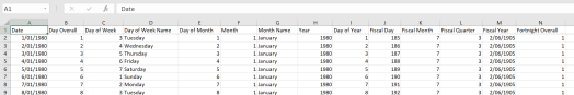
As promised, the code to populate these fields;
Day Overall: start at 1 and fill down
Day of Week: =WEEKDAY(A2)
Day of Week Name: =TEXT(A2, “dddd”)
Day of Month: =DAY(A2)
Month: =MONTH(A2)
Month Name: =TEXT(A2, “mmmm”)
Year: =YEAR(A2)
Day Of Year: =A2-DATE(H2,1,1)+1
Fiscal Day: =A2-DATE(H2+(F2<7)*-1,7,1)+1
Fiscal Month: =CHOOSE(F2,7,8,9,10,11,12,1,2,3,4,5,6)
Fiscal Quarter: =FLOOR((K2-1)/3,1)+1
Fiscal Year: =YEAR(A2)+(MONTH(A2)>6)
Fortnight: =FLOOR(B2/14,1)+1
Important note, in Australia our fiscal year runs July 1 – June 30
Are you having fun yet? Feel free to add more columns as required for your particular applications.
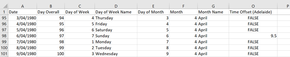
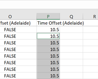
Now comes the slightly curly bit – adding the time zones in. If you’re in a location in which there is no daylight savings, congratulations! You can just add the time zone offset, fill down, and away we go. Me in Adelaide? I have a bit more work to do. Our time zone changes on the first Sunday in April, and the first Sunday in October. Wouldn’t want to make it a consistent date would we, that’d be far too easy. So first we have to identify those days, which we can do fairly easily with a bulky and not at all elegant collection of IF statements:
=IF(D2=”Sunday”,IF(E2<=7,IF(G2=”April”,9.5,IF(G2=”October”,10.5))))
This fills our new Time Zone Offset column with a bunch of FALSEs, except on the first Sunday of April and October:
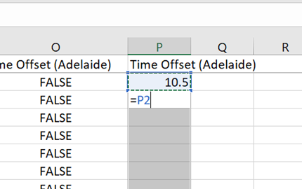
From here we can copy and paste the values (right click -> paste values so we don’t maintain the formulas) into a new column. We should also replace the top value (P2 in this example) with the expected time offset as we’ll be filling down. CTRL+H to find and replace all of the ‘FALSE’ values with blank, which we can then select by highlighting the entire new column and going to Home -> Find & Select -> Go To Special -> Blanksand hitting OK. Now we have all of the blank values highlighted, we’re going to fill down by entering the formula which will pull from the value above it, and hitting CTRL+Enterto fill the cells likewise:
We now should have an accurate time zone offset for every day in our table! Go ahead and save a copy as a csv for use wherever you need. This still doesn’t help me in Power BI
As mentioned above, there are perfectly valid ways to do this dynamically in Power BI. And I can already hear you thinking ‘The connection to a CSV is going to break immediately if it’s not hosted in Sharepoint or otherwise’. Fear not, because we’re not actually going to use the CSV past it being an original source – this is the reason we’ve thus far done everything outside of Power BI. If you’re still confused don’t worry, it’ll all become clear momentarily.
Static Date Dimension in Power BI
As mentioned above, a connection to a CSV in Power BI is almost always a bad play. We also don’t want to use time, energy, and resources unnecessarily to refresh something that is very unlikely to change (because you’ve already communicated with the wider business and established the scope of date filtering needs right?). So the best case scenario would be to have this dimension just contained in the Power BI report, unchanging and useful. We can do this with small amounts of data by utilizing the ‘Enter Data’ functionality, but that’s limited to 3000 rows – we need much more than that. Luckily, with most things tech-related there’s a workaround! (Author’s note: the following process reminds me a bit of the Quake fast inverse square root – if you don’t know what that is and you like stories of when tech and black magic meet it’s worth a Google)
Step 1 – Open Power BI and import
This should be fairly basic, we’re going to open a new report in Power BI and import our CSV into the Power Query Editor. The table created should match the name of the CSV, if it doesn’t then either rename or take note of it, we’re going to use it in the next step.
Step 2 – Magic M conversions
We’re now going to create a new blank query and enter the following M code into the formula bar:
= Text.From( Binary.Compress( Binary.FromText( Text.From( Json.FromValue( <TABLE_NAME_FROM_PREVIOUS_STEP_GOES_HERE> ) ), BinaryEncoding.Base64 ), Compression.GZip ) )
This is going to populate a bunch of characters that match what I would expect the output of 1000 monkeys on 1000 typewrites would be if they were properly caffeinated. Don’t panic, this is part of the process:
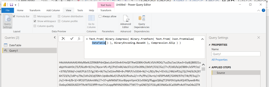
You will be able to copy directly from the Power Query window, so go ahead and grab that colossal wall of text
Step 3 – Make the elephant reappear!
Once we have our gigantic wall of text we’re going to go back into the Power Query Editor and create a new blank query again, containing the following M:
= Json.Document( Text.FromBinary( Binary.Decompress( Binary.FromText( “<MASSIVE_WALL_OF_TEXT_GOES_HERE>” ), Compression.GZip ) ) )
If you’ve appropriately aligned your pentagram you should be presented with your date table back (after the appropriate expansion from a list):
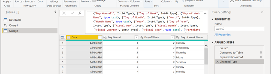
This data is totally self-hosted in Power BI, independent of any connections, and 100% portable. We can now delete the first two queries (DateTable and Query1), rename our final Date Dimension Table and save.
Side notes: this works for all data, and I believe it’s technically limitless. Of course practically there is a limit, but since it’s performance-independent you’re mostly going to be constrained by how unwieldy the file size gets (though for most applications the date tables are some of the smallest pieces of data). Additionally, because this is held within the Power BI file you can no longer Connect Live to Datasets in the Power BI Service, so if you’re doing composite modelling you’ll need to create these at the same time as you do your other Extract & Load. There are a heap of business applications that this technique may be applicable for – static dimensions are great candidates. Doing so can greatly reduce the amount of data needing to be consumed from source systems, and will likely reduce refresh times accordingly.
What time is it?
All of this and we still really haven’t touched on the crux of the problem, which is that Power BI Service isn’t maintaining my time zone. We best address that.
In all of my reports I include two measures; the datetime the data was last refreshed, and the datetime the report was created. The former is generated by another query in the Power Query editor, as follows:
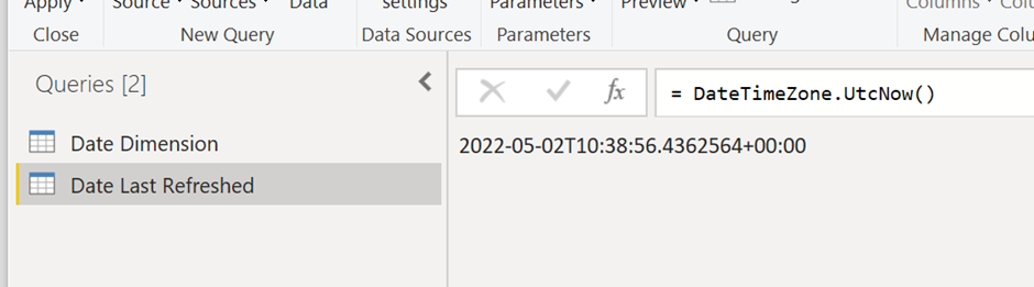
And the latter is just a measure made in DAX. When we create these measures if we left them unadjusted they would appear fine in our development environment, because Microsoft is pulling from our system settings to apply offsets. But as soon as we publish to Power BI Service, that’s going to be shifted back to UTC. We now have in our Date Dimension the offset, so we can utilize that to adjust the times – all we need to do is lookup what the offset should be for today.
The measures I typically create are relatively straightforward. For ease of comprehension, I typically do the lookup in a separate measure, as follows:
Time offset = LOOKUPVALUE(‘Date Dimension'[Time Offset (Adelaide)],’Date Dimension'[Date],UTCTODAY())/24
The important thing to note here is that the value returned by the lookup needs to be divided by 24 to give an offset that can be applied to a datetime. From there it’s simple to create the accurate refresh measures:
Date Last Refreshed = “Data Last Refreshed: ” & FORMAT(LASTDATE(‘Date Last Refreshed'[Column1]) + [Time offset], “yyyy-MM-dd h:mm AMPM”)
Report Generation Date (Adjusted) = “Report Generated: ” & FORMAT(UTCNOW() + [Time offset], “dd/MM/yyyy h:mm AMPM”)
And publishing to Power BI Service we can see that the refresh times match the local timezone:
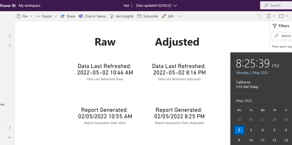
There are of course limitations to this approach. Consumers in a different time zone will still have the report not match their local time with this basic implementation – more advanced implementations with user-specific RLS can be much better. But for the simple purpose of giving your users an understanding of how fresh the information they’re viewing is, this is a very tidy way to do so.